ResoKit’s Tutorial

This tutorial is a guide to use ResoKit package. ResoKit is toolkit package for the analysis and diagnostics exoplanetary planetary systems.

In this tutorial we show, step by step, how to get started with the ResoKit package.

---

Import ResoKit and the necessary packages

import resokit

Loading the data

The first step is to load an exoplanetary system. The available datasets are NASA or EU. Both datasets are provided with the package, and they can be updated if necessary.

To load a system, functions from_nasa and from_eu are provided in the load module.

For this tutorial, we will work with the Kepler-47 exoplanetary system, from the Exoplanet.eu dataset.

Remember to download the datasets first. See the datasets tutorial for more information.

kepler47 = resokit.load.from_eu("Kepler-47", soft=True)

Looking for star system 'Kepler-47' in eu database.
 Loading the entire dataset...
  Reading exoplanet_eu.csv directly from /home/egianuzzi/.resokit_data/exoplanet_eu.zip...
Updated stored index in memory.
Stored dataset in memory.
 Found a very close star match: 'Kepler-47 A' in eu dataset.
 Execute with exact_match=False to load it, or rewrite the name.

Note: If we set soft=False (default), a ValueError is raised if the system is not found.

If the system (or star in this case) name is entered incorrectly, ResoKit will attempt to detect the intended system and provide suggestions based on it. As Exoplanet.eu is indexed through star name, we see here that the correct system (star) name is Kepler-47 A.

kepler47 = resokit.load.from_eu("Kepler-47 A")

Looking for star system 'Kepler-47 A' in eu database.
 Loaded full dataset from memory stored datasets.
Checking if 'Kepler-47 A' is a binary system...
 Found a very close binary match in: ['Kepler47']
 Execute with exact_match=False to load it.
Star Kepler-47 A could be part of a binary system.
Creating system 'Kepler-47'.
 Star 'Kepler-47 A' created.
 3 planets created.

It seems that Kepler-47 is a binary star system, so we wil try then to load the system using exact_match=False.

The main problem is that both databases have different star and system names, but using exact_match=False an approximate link between them will be done.

In this case we can remove the “ A”, and keep the hyphen “-“.

kepler47 = resokit.load.from_eu("Kepler-47", exact_match=False)

Looking for star system 'Kepler-47' in eu database.
 Loaded full dataset from memory stored datasets.
 Found a very close star match: 'Kepler-47 A' in eu dataset.
 Loading the almost exact match...
Checking if 'Kepler-47 A' is a binary system...
 Binary system found in ['Kepler47'], in p-type binary orbit.
Creating system 'Kepler-47'.
 Using binary star 'Kepler-47'.
 3 planets created.

Now, kepler47 is a Static System; and we also know that it is a circumbinary planets system.

We can see its components (star and planets) and where the system was obtained from.

kepler47

StaticSystem: 'Kepler-47'
 Star 1:
  Kepler-47 A
 Star 2:
  Kepler-47 B
 Planets:
  Kepler-47 (AB)b
  Kepler-47 (AB)d
  Kepler-47 (AB)c
 [circumbinary system]
from 'eu' data source.

Note:

Just in case we do not want the system to be a binary star system (even though it is), we can execute the previous with check_binary=False.

resokit.load.from_eu("Kepler-47", exact_match=False, check_binary=False)

Looking for star system 'Kepler-47' in eu database.
 Loaded full dataset from memory stored datasets.
 Found a very close star match: 'Kepler-47 A' in eu dataset.
 Loading the almost exact match...
Creating system 'Kepler-47'.
 Star 'Kepler-47 A' created.
 3 planets created.

StaticSystem: 'Kepler-47 A'
 Star:
  Kepler-47 A
 Planets:
  Kepler-47 (AB)b
  Kepler-47 (AB)d
  Kepler-47 (AB)c
from 'eu' data source.

Analysing the Static System

Some features we can apply to this System are:

• System planets parameters: get_item

• Individual planet inspection: planet

• Calculate period ratios: period_ratios

• Plot planet, star, of general system attributes: plot

• Remove or add a planet: remove, add

We will now explain how to use each of them.

Inspection

We can access the parameters of every planet as if it were a dataframe, though the slice method

For example the mass

kepler47["mass"]

Kepler-47 (AB)b        NaN
Kepler-47 (AB)d    0.05984
Kepler-47 (AB)c        NaN
Name: mass, dtype: float64

Or the radius and the Period

kepler47[["radius", "P"]]

	radius	P
Kepler-47 (AB)b	0.2700	49.514
Kepler-47 (AB)d	0.6281	187.350
Kepler-47 (AB)c	0.4100	303.148

Another method is using the get_item method.

For example, for the eccentricity and inclination; and its errors too!

kepler47.get_item(["e", "inc"], error=True)

	e	e_err_min	e_err_max	inc	inc_err_min	inc_err_max
Kepler-47 (AB)b	NaN	NaN	NaN	89.590	0.5	0.5
Kepler-47 (AB)d	0.024	0.017	0.025	90.000	NaN	NaN
Kepler-47 (AB)c	NaN	NaN	NaN	89.826	NaN	NaN

Planet access

We can access any planet (or even the system star) from the Static System.

For example, if we want to retrieve the 2nd planet (sorted by period), we simply do

planet2 = kepler47.planet(1) # Remember python is 0 indexed, so the second planet is "1".
planet2

	4745
mass_err_max	0.0749
tperi_err_min	NaN
a_err_max	0.0033
e_err_min	0.017
inc	90.0
w_err_min	166.0
a_err_min	0.0033
tperi_err_max	NaN
mass_sin_i	NaN
disc_method	Timing
name	Kepler-47 (AB)d
mass_sin_i_err_min	NaN
n	0.033537
rowupdate	2024-08-12
inc_err_max	NaN
e	0.024
P_err_min	0.15
radius	0.6281
radius_err_min	0.0437
star_name	Kepler-47 A
radius_err_max	0.0589
a	0.6992
tperi	NaN
inc_err_min	NaN
P_err_max	0.15
w	352.0
w_err_max	96.0
e_err_max	0.025
n_err_min	41.887902
mass_err_min	0.0368
disc_year	2013.0
mass	0.05984
reference	Published in a refereed paper
mass_sin_i_err_max	NaN
P	187.35
n_err_max	41.887902

StaticPlanet 'Kepler-47 (AB)d'' from eu data source - 1 row x 36 columns

We can display the planet properties as a Series.

planet2.data

mass_err_max                                 0.0749
tperi_err_min                                   NaN
a_err_max                                    0.0033
e_err_min                                     0.017
inc                                            90.0
w_err_min                                     166.0
a_err_min                                    0.0033
tperi_err_max                                   NaN
mass_sin_i                                      NaN
disc_method                                  Timing
name                                Kepler-47 (AB)d
mass_sin_i_err_min                              NaN
n                                          0.033537
rowupdate                                2024-08-12
inc_err_max                                     NaN
e                                             0.024
P_err_min                                      0.15
radius                                       0.6281
radius_err_min                               0.0437
star_name                               Kepler-47 A
radius_err_max                               0.0589
a                                            0.6992
tperi                                           NaN
inc_err_min                                     NaN
P_err_max                                      0.15
w                                             352.0
w_err_max                                      96.0
e_err_max                                     0.025
n_err_min                                 41.887902
mass_err_min                                 0.0368
disc_year                                    2013.0
mass                                        0.05984
reference             Published in a refereed paper
mass_sin_i_err_max                              NaN
P                                            187.35
n_err_max                                 41.887902
Name: 4745, dtype: object

And we can access any of this attributes. For example the name, or the semi-major axis a:

planet2.name

'Kepler-47 (AB)d'

planet2.a

0.6992

Just, remember the main units! Semimajor-axis (\(a\)) is in Astronomical Units.

Calculate and plot (if possible) period ratios

If we want to obtain the period ratio between all pair of planets: \(P_{i+1}/P_{i}\), we simply invoke Static System period_ratios_ attribute.

kepler47.period_ratios_

	Kepler-47 B	Kepler-47 (AB)b	Kepler-47 (AB)d	Kepler-47 (AB)c
Kepler-47 B	1.000000	5.729266	21.678272	35.077261
Kepler-47 (AB)b	0.174542	1.000000	3.783778	6.122470
Kepler-47 (AB)d	0.046129	0.264286	1.000000	1.618084
Kepler-47 (AB)c	0.028508	0.163333	0.618015	1.000000

Here we can see that \(P_\textnormal{Kepler-47 (AB)c} \sim 6.122470 \times P_\textnormal{Kepler-47 (AB)b}\) .

If we want to get the period ratios as fractions, we simply invoke Static System period_ratio method, including (if wanted) any resokit.utils.float_to_fraction function argument inside a dict named fraction_kwargs. For example: max_error (which is the maximum relative error between the estimated fraction and the floating period ratio).

kepler47.period_ratio("all", use_binary=False, fraction_kwargs={"max_error":1e-1})

Approximating float 1.000000 as a continued fraction:
 Iter  1:   1/1   -> 1.000000 (error: 0.00e+00)
Approximating float 0.264286 as a continued fraction:
 Iter  1:   0/1   -> 0.000000 (error: 1.00e+00)
 Iter  2:   1/3   -> 0.333333 (error: 2.61e-01)
 Iter  3:   1/4   -> 0.250000 (error: 5.41e-02)
Approximating float 0.163333 as a continued fraction:
 Iter  1:   0/1   -> 0.000000 (error: 1.00e+00)
 Iter  2:   1/6   -> 0.166667 (error: 2.04e-02)
Approximating float 3.783778 as a continued fraction:
 Iter  1:   3/1   -> 3.000000 (error: 2.07e-01)
 Iter  2:   4/1   -> 4.000000 (error: 5.71e-02)
Approximating float 1.000000 as a continued fraction:
 Iter  1:   1/1   -> 1.000000 (error: 0.00e+00)
Approximating float 0.618015 as a continued fraction:
 Iter  1:   0/1   -> 0.000000 (error: 1.00e+00)
 Iter  2:   1/1   -> 1.000000 (error: 6.18e-01)
 Iter  3:   1/2   -> 0.500000 (error: 1.91e-01)
 Iter  4:   2/3   -> 0.666667 (error: 7.87e-02)
Approximating float 6.122470 as a continued fraction:
 Iter  1:   6/1   -> 6.000000 (error: 2.00e-02)
Approximating float 1.618084 as a continued fraction:
 Iter  1:   1/1   -> 1.000000 (error: 3.82e-01)
 Iter  2:   2/1   -> 2.000000 (error: 2.36e-01)
 Iter  3:   3/2   -> 1.500000 (error: 7.30e-02)
Approximating float 1.000000 as a continued fraction:
 Iter  1:   1/1   -> 1.000000 (error: 0.00e+00)

	Kepler-47 (AB)b	Kepler-47 (AB)d	Kepler-47 (AB)c
Kepler-47 (AB)b	(1, 1)	(4, 1)	(6, 1)
Kepler-47 (AB)d	(1, 4)	(1, 1)	(3, 2)
Kepler-47 (AB)c	(1, 6)	(2, 3)	(1, 1)

Here, is more clear that \(P_\textnormal{Kepler-47 (AB)b}\) and \(P_\textnormal{Kepler-47 (AB)c}\) are somewhat close to a \(6/1\) mean motion resonance. Moreover, we also see that \(P_\textnormal{Kepler-47 (AB)d}\) and \(P_\textnormal{Kepler-47 (AB)c}\) are somewhat close to a \(3/2\) mean motion resonance.

In case the errors (of the period ratio estimations) are needed, they can be obtained invoking Static System period_ratio method again, with errors=True. They are calculated using each observed period error, so each value is an upper limit for the error.

Here we also calculate the error for the period ratios including the binary star.

kepler47.period_ratio(error=True)

	Kepler-47 B	Kepler-47 (AB)b	Kepler-47 (AB)d	Kepler-47 (AB)c
Kepler-47 B	NaN	NaN	NaN	NaN
Kepler-47 (AB)b	NaN	0.001142	0.004304	0.005155
Kepler-47 (AB)d	NaN	0.000301	0.001132	0.001351
Kepler-47 (AB)c	NaN	0.000138	0.000516	0.000336

As expected, the errors related to the binary star are NaN because the binary period has no errors set.

Plot the period ratios

If the system has a triplet (three planets or more), it can be plotted in a period ratios separations space: \(P_{i+1}/P_{i}\) vs. \(P_{i+2}/P_{i+1}\). To do so, we invoke Static System plot_triplet method. Here, we also plot the errors.

ax = kepler47.plot_triplet(error=True, capsize=10)
ax.legend()
ax.set_xlabel("Period Ratio ($P_2/P_1$)")
ax.set_ylabel("Period Ratio ($P_3/P_2$)")

Text(0, 0.5, 'Period Ratio ($P_3/P_2$)')

Note: The binary is not included in these triplet plots (yet).

If we want more manual operation at plotting 3-body mean motion resonances near the system triplets, we can invoke the resokit.utils.mmr.plot_mmrs method. Also, we set draw_mmr=False to avoid plotting them twice.

This method will plot the resonances that are near the triplets.

Note: It its highly recommended to set the axes limits (xlim and ylim) before calling plot_mmrs, especially if label_mmrs=True.

bounds = [2.51, 4.5, 1.41, 2.1]  # [xmin, xmax, ymin, ymax]
ax = kepler47.plot_triplet(error=True, capsize=10, label=True, draw_mmr=False)
ax.set_xlim(bounds[0], bounds[1])
ax.set_ylim(bounds[2], bounds[3])
resokit.utils.mmr.plot_mmrs(
    bounds=bounds,
    ax=ax,
    label_mmrs=True,
    color="black",
    )
ax.legend()
ax.set_xlabel("Period Ratio ($P_2/P_1$)")
ax.set_ylabel("Period Ratio ($P_3/P_2$)")

Text(0, 0.5, 'Period Ratio ($P_3/P_2$)')

Here, the 3-body resonances are annotated with the corresponding period ratios.

Plot system attributes

We can plot any pair attributes of the StaticSystem, of any planet in the system.

ax = kepler47.plot("mass", "radius", error_x=True, error_y=True)
ax.legend()
ax.set_xlabel("Mass ($M_J$)")
ax.set_ylabel("Radius ($R_J$)")

Text(0, 0.5, 'Radius ($R_J$)')

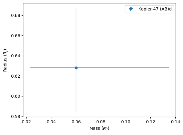
Some planets are not plotted because they do not have both requested attributes measured.

For example, in this case…

kepler47["radius"]

Kepler-47 (AB)b    0.2700
Kepler-47 (AB)d    0.6281
Kepler-47 (AB)c    0.4100
Name: radius, dtype: float64

We see the three planets have radius estimations; but…

kepler47["mass"]

Kepler-47 (AB)b        NaN
Kepler-47 (AB)d    0.05984
Kepler-47 (AB)c        NaN
Name: mass, dtype: float64

only Kepler-47 (AB)d has its mass estimated.

Estimations

To solve this problem, ResoKit also provides tools for mass (or radius) estimation with diverse models, from the estimated radius (or mass).

To do so, we simply use estimate_mass function.

kepler47.estimate_mass()

Kepler-47 (AB)b    0.028559
Kepler-47 (AB)d    0.059840
Kepler-47 (AB)c    0.058045
Name: mass, dtype: float64

Here we used the default estimate_mass parameters, but we can get different estimations with different models, and also include the errors.

kepler47.estimate_mass(model="m24", err_method=2)

	mass	mass_err_min	mass_err_max
Kepler-47 (AB)b	0.037816	0.002276	0.002322
Kepler-47 (AB)d	0.059840	0.036800	0.074900
Kepler-47 (AB)c	0.070543	0.004572	0.004672

The models available for mass-radius relations are:

• ‘ck17’: Chen & Kipping (2017) [trivariate] (Naive approximation)

• ‘o20’: Otegi et al. (2020) [density|bivariate]

• ‘e23’: Edmondson et al. (2023)

• ‘m24’: Müller et al. (2024) [bivariate]

Remove or add planets

Remove

To remove a planet, we can simply invoke the remove_planet method of StaticSystem.

modified_kepler47 = kepler47.remove_planet(2)  # Remember python is 0 indexed, so the third planet is "2".
modified_kepler47

Planet Kepler-47 (AB)c [2] removed.

StaticSystem: 'Kepler-47'
 Star 1:
  Kepler-47 A
 Star 2:
  Kepler-47 B
 Planets:
  Kepler-47 (AB)b
  Kepler-47 (AB)d
 [circumbinary system]
from 'eu' data source.

We can also remove planets by suffix.

modified_kepler47.suffixes_

['A', 'B', 'b', 'd']

modified_kepler47 = kepler47.remove_planet("b")
modified_kepler47

Planet Kepler-47 (AB)b [0] removed.

StaticSystem: 'Kepler-47'
 Star 1:
  Kepler-47 A
 Star 2:
  Kepler-47 B
 Planets:
  Kepler-47 (AB)d
  Kepler-47 (AB)c
 [circumbinary system]
from 'eu' data source.

# We check that the number of planets has been reduced
modified_kepler47.n_planets_

2

We can look the new system metadata, and we will find that ‘removed_planet’ has been added. Also some extra information can be found…

for k,v in modified_kepler47.metadata.items():
    print(k, v)

ResoKit 0.1.dev289
author Emmanuel Gianuzzi
author_email egianuzzi@unc.edu.ar
affiliation FAMAF-IATE-OAC-CONICET
platform Linux-6.8.0-65-generic-x86_64-with-glibc2.35
system_encoding utf-8
python 3.10.12 (main, May 27 2025, 17:12:29) [GCC 11.4.0]
license MIT
load_system Kepler-47
eu_indexes [4744, 4745, 4743]
removed_planet ['Kepler-47 (AB)b']

Add

To add a planet, we can simply invoke the add_planet method of StaticSystem.

# Get a planet from the original system
planet2 = kepler47.planet(1)  # Remember python is 0 indexed, so the second planet is "1".

# Add the planet to the modified system
modified_kepler47.add_planet(planet2)

Planet Kepler-47 (AB)d added.

<attrs generated methods resokit.core.StaticSystem>:31: UserWarning: Planets must have unique names.
  self.__attrs_post_init__()

StaticSystem: 'Kepler-47'
 Star 1:
  Kepler-47 A
 Star 2:
  Kepler-47 B
 Planets:
  Kepler-47 (AB)d
  Kepler-47 (AB)d
  Kepler-47 (AB)c
 [circumbinary system]
from 'eu' data source.

Here, we added a planet that already exists in the system, so a Warning was raised.

If a planet not existing in the system is added, no warning will be raised.

# Extract the planet 2 from the original system
planet2 = kepler47.planet(1)  # Remember python is 0 indexed, so the second planet is "1".

# Remove the planet from the original system
modified_kepler47 = kepler47.remove_planet(1)

# Add again the planet to the modified system
modified_kepler47 = modified_kepler47.add_planet(planet2)

# Check that the planet has been added
modified_kepler47

Planet Kepler-47 (AB)d [1] removed.
Planet Kepler-47 (AB)d added.

StaticSystem: 'Kepler-47'
 Star 1:
  Kepler-47 A
 Star 2:
  Kepler-47 B
 Planets:
  Kepler-47 (AB)b
  Kepler-47 (AB)d
  Kepler-47 (AB)c
 [circumbinary system]
from 'eu' data source.

Replace

Another feature possible to do with this StaticSystem is to replace a planet with another.

Lets take for example Kepler-47 (AB)b.

kepler47_b = kepler47.planet("b")
kepler47_b

	4743
mass_err_max	NaN
tperi_err_min	NaN
a_err_max	0.0047
e_err_min	NaN
inc	89.59
w_err_min	NaN
a_err_min	0.0047
tperi_err_max	NaN
mass_sin_i	NaN
disc_method	Primary Transit
name	Kepler-47 (AB)b
mass_sin_i_err_min	NaN
n	0.126897
rowupdate	2024-08-12
inc_err_max	0.5
e	NaN
P_err_min	0.04
radius	0.27
radius_err_min	0.011
star_name	Kepler-47 A
radius_err_max	0.011
a	0.2956
tperi	NaN
inc_err_min	0.5
P_err_max	0.04
w	NaN
w_err_max	NaN
e_err_max	NaN
n_err_min	157.079633
mass_err_min	NaN
disc_year	2012.0
mass	NaN
reference	Published in a refereed paper
mass_sin_i_err_max	NaN
P	49.514
n_err_max	157.079633

StaticPlanet 'Kepler-47 (AB)b'' from eu data source - 1 row x 36 columns

We see again that this planet doesn’t have its mass measured…

but we can estimate it and create a new planet with the estimated mass.

new_kepler47_b = kepler47_b.estimate_mass(new_planet=True)
new_kepler47_b.mass

np.float64(0.028559320687648843)

We can see the modified metadata of this new planet.

for k,v in new_kepler47_b.metadata.items():
    print(k, v)

ResoKit 0.1.dev289
author Emmanuel Gianuzzi
author_email egianuzzi@unc.edu.ar
affiliation FAMAF-IATE-OAC-CONICET
platform Linux-6.8.0-65-generic-x86_64-with-glibc2.35
system_encoding utf-8
python 3.10.12 (main, May 27 2025, 17:12:29) [GCC 11.4.0]
license MIT
load_system Kepler-47
eu_indexes 4743
history ['Added mass to 0.028559320687648843.']

Now, we can replace the old b planet with the new one using replace.

new_kepler47 = kepler47.replace_planet("b", new_kepler47_b)
new_kepler47

Planet Kepler-47 (AB)b [0] replaced by Kepler-47 (AB)b.

StaticSystem: 'Kepler-47'
 Star 1:
  Kepler-47 A
 Star 2:
  Kepler-47 B
 Planets:
  Kepler-47 (AB)b
  Kepler-47 (AB)d
  Kepler-47 (AB)c
 [circumbinary system]

We can verify the mass of the new planet.

new_kepler47.get_item("mass")

Kepler-47 (AB)b    0.028559
Kepler-47 (AB)d    0.059840
Kepler-47 (AB)c         NaN
Name: mass, dtype: float64

Finally, as expected, the metadata and source of the new system has also changed from the original.

print("Old source:", kepler47.source_)
print("New source:", new_kepler47.source_)

print("Metadata:")
for k,v in new_kepler47.metadata.items():
    print(k, v)

Old source: eu
New source: user
Metadata:
ResoKit 0.1.dev289
author Emmanuel Gianuzzi
author_email egianuzzi@unc.edu.ar
affiliation FAMAF-IATE-OAC-CONICET
platform Linux-6.8.0-65-generic-x86_64-with-glibc2.35
system_encoding utf-8
python 3.10.12 (main, May 27 2025, 17:12:29) [GCC 11.4.0]
license MIT
load_system Kepler-47
eu_indexes [4744, 4745, 4743]
changed_planet ['Kepler-47 (AB)b']